Examples

The Examples folder contains example scripts (!) of how SciScripts can be used for experiments and analysis. Here is a walkthrough for the Examples/FilteringAndPlotting.py script.

Load data from an open-ephys recording folder:

In [1]: import numpy as np

In [2]: from sciscripts.IO import IO

In [3]: from sciscripts.Analysis import Analysis

In [4]: from sciscripts.Analysis.Plot import Plot

In [5]: Folder = 'DataSet/2018-08-13_13-25-45_1416'

In [6]: Data, Rate = IO.DataLoader(Folder)

Loading recording1 ...
Loading recording2 ...
Loading recording3 ...
Loading recording4 ...
Loading recording5 ...
Loading recording6 ...
Loading recording7 ...
Loading recording8 ...
Converting to uV...

Select a recording and filter it:

In [7]: Proc = list(Data.keys())[0]             # Select 1st rec processor

In [8]: DataExp = list(Data[Proc].keys())[0]    # Select 1st experiment

In [9]: Rec0 = Data[Proc][DataExp]['0'][:,:8]   # Select the 1st 8 channels

In [10]: Rate0 = Rate[Proc][DataExp]

In [11]: Time0 = np.arange(Rec0.shape[0])/Rate0

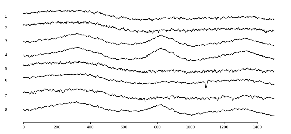
Plot 50ms of raw channels:

In [12]: Plot.AllCh(Rec0[:int(Rate0*0.05),:], Save=True, File='Plot1', Ext=['png'])

Filtering in theta and gamma bands:

In [13]: Rec0Theta = Analysis.FilterSignal(Rec0, Rate0, Frequency=[4,12], Order=2)
Filtering channel 1 ...
Filtering channel 2 ...
Filtering channel 3 ...
Filtering channel 4 ...
Filtering channel 5 ...
Filtering channel 6 ...
Filtering channel 7 ...
Filtering channel 8 ...

In [14]: Rec0Gamma = Analysis.FilterSignal(Rec0, Rate0, Frequency=[30,100], Order=3)
Filtering channel 1 ...
Filtering channel 2 ...
Filtering channel 3 ...
Filtering channel 4 ...
Filtering channel 5 ...
Filtering channel 6 ...
Filtering channel 7 ...
Filtering channel 8 ...

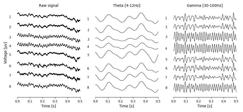
Plot raw, theta and gamma:

In [15]: Window = int(Rate0/2)
    ...: plt = Plot.plt # This is exactly the same as `import matplotlib.pyplot as plt`
    ...: Fig, Axes = plt.subplots(1,3)
    ...: Axes[0] = Plot.AllCh(Rec0[:Window,:], Time0[:Window], Ax=Axes[0], lw=0.7)
    ...: Axes[1] = Plot.AllCh(Rec0Theta[:Window,:], Time0[:Window], Ax=Axes[1], lw=0.7)
    ...: Axes[2] = Plot.AllCh(Rec0Gamma[:Window,:], Time0[:Window], Ax=Axes[2], lw=0.7)
    ...:
    ...: AxArgs = {'xlabel': 'Time [s]'}
    ...: for Ax in Axes: Plot.Set(Ax=Ax, AxArgs=AxArgs)
    ...:
    ...: Axes[0].set_ylabel('Voltage [µv]')
    ...: Axes[0].set_title('Raw signal')
    ...: Axes[1].set_title('Theta [4-12Hz]')
    ...: Axes[2].set_title('Gamma [30-100Hz]')
    ...:
    ...: Plot.Set(Fig=Fig) # apply tight layout and hide fig patch
    ...: Fig.savefig('Plot2.png')
    ...: plt.show()

More scripts using this package for real experiments and analysis can be found at Examples.